
Have you ever found yourself struggling to make sense of your data because it’s not presented in an easily digestible format? That feeling is common in the realm of data science, where knowing how to reshape and merge datasets can significantly enhance your analysis. In this article, we’ll delve into the essential techniques of data reshaping and merging, particularly focusing on melting, pivoting, and joining data. By the end, you’ll have a solid understanding of how to manipulate your data effectively.
Understanding Data Reshaping
Data reshaping refers to changing the layout of your data to make it more suitable for analysis. This process is vital because different analyses may require data to be arranged in specific formats. You might need to convert a wide format to a long format or vice versa, depending on your purposes.
Why Reshape Data?
You might wonder why reshaping data is necessary. Here are a few reasons:
-
Analytical Compatibility: Different statistical models and plots require data in certain formats. For instance, a time series analysis might call for a long format where each time point is a separate row.
-
Ease of Interpretation: Users can find it easier to interpret data when it’s presented clearly. This clarity allows for faster insights and decision-making.
-
Visualization Needs: Many plotting libraries expect data in specific shapes. Reshaping ensures that you can render the graphics you need effectively.
")
Techniques of Data Reshaping
There are several techniques for reshaping data, but we will focus on three primary methods: melting, pivoting, and joining. Each of these methods serves unique purposes and can help you manipulate your datasets more efficiently.
Melting Data
Melting is the process of transforming a DataFrame from a wide format to a long format. In a wide format, variables are spread across multiple columns, while a long format has a single column for variable names and another for their respective values. Melting is particularly useful for simplifying datasets.
When to Use Melting?
You will find melting beneficial when:
- You have multiple measurement variables stored in different columns.
- You need to aggregate or plot data easily across different categories.
How to Melt Data?
Let’s look at a simple example. Suppose you have a DataFrame that tracks sales for different products over several months:
| Product | Jan | Feb | Mar |
|---|---|---|---|
| A | 100 | 150 | 200 |
| B | 80 | 90 | 100 |
| C | 150 | 200 | 250 |
To melt this DataFrame, you would convert it into a format like this:
| Product | Month | Sales |
|---|---|---|
| A | Jan | 100 |
| A | Feb | 150 |
| A | Mar | 200 |
| B | Jan | 80 |
| B | Feb | 90 |
| B | Mar | 100 |
| C | Jan | 150 |
| C | Feb | 200 |
| C | Mar | 250 |
Melting in Python
If you’re using Python and Pandas, melting can be done easily using the melt function:
import pandas as pd
Sample DataFrame
data = { ‘Product’: [‘A’, ‘B’, ‘C’], ‘Jan’: [100, 80, 150], ‘Feb’: [150, 90, 200], ‘Mar’: [200, 100, 250] } df = pd.DataFrame(data)
Melting the DataFrame
melted_df = df.melt(id_vars=[‘Product’], var_name=’Month’, value_name=’Sales’) print(melted_df)
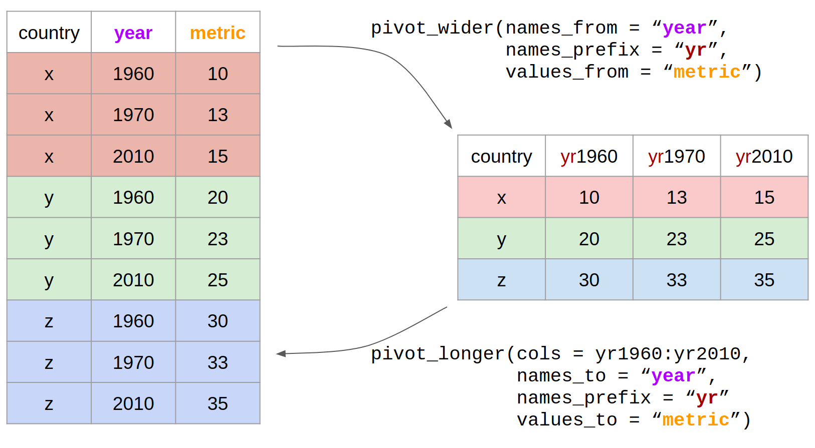
Pivoting Data
While melting is all about turning wide data into long data, pivoting does the opposite. Pivoting allows you to reorganize your data by transforming unique values from one column into multiple columns across the DataFrame.
When to Use Pivoting?
Pivoting shines in scenarios where you have categorical data and you want to create a summary table that showcases multiple data points across various categories.
How to Pivot Data?
Consider a simple sales record example:
| Product | Month | Sales |
|---|---|---|
| A | Jan | 100 |
| A | Feb | 150 |
| B | Jan | 80 |
| B | Feb | 90 |
You might want to pivot this data so that each product has its monthly sales represented across distinct columns:
| Product | Jan | Feb |
|---|---|---|
| A | 100 | 150 |
| B | 80 | 90 |
Pivoting in Python
In Pandas, you can pivot data using the pivot function:
Sample DataFrame
data = { ‘Product’: [‘A’, ‘A’, ‘B’, ‘B’], ‘Month’: [‘Jan’, ‘Feb’, ‘Jan’, ‘Feb’], ‘Sales’: [100, 150, 80, 90] } df = pd.DataFrame(data)
Pivoting the DataFrame
pivoted_df = df.pivot(index=’Product’, columns=’Month’, values=’Sales’) print(pivoted_df)
Joining Data
Joining data involves combining two or more datasets based on common keys or indexes. This technique is fundamental for consolidating information from different sources into a single coherent set.
Types of Joins
When you perform a join, you can use several different strategies, including:
- Inner Join: Returns only the rows with matching values in both datasets.
- Outer Join: Includes all rows from either dataset, filling in with NaNs where no match exists.
- Left Join: Returns all rows from the left dataset and the matched rows from the right dataset.
- Right Join: Returns all rows from the right dataset and the matched rows from the left dataset.
When to Use Joins?
You might want to join datasets when:
- You need to augment your primary dataset with additional information from another source.
- You have separate datasets that share common identifiers, like a user ID.
How to Join Data?
Let’s say you have two datasets: one for product information and another for sales.
Product Data:
| ProductID | ProductName |
|---|---|
| 1 | Widget A |
| 2 | Widget B |
| 3 | Widget C |
Sales Data:
| SalesID | ProductID | Amount |
|---|---|---|
| 101 | 1 | 100 |
| 102 | 2 | 150 |
| 103 | 1 | 200 |
You might want to join these two tables based on ProductID to create a comprehensive sales report:
Joined Data:
| SalesID | ProductID | Amount | ProductName |
|---|---|---|---|
| 101 | 1 | 100 | Widget A |
| 102 | 2 | 150 | Widget B |
| 103 | 1 | 200 | Widget A |
Joining in Python
Using Pandas, you can perform a join with the merge function. Here’s how:
Sample DataFrames
product_data = { ‘ProductID’: [1, 2, 3], ‘ProductName’: [‘Widget A’, ‘Widget B’, ‘Widget C’] } sales_data = { ‘SalesID’: [101, 102, 103], ‘ProductID’: [1, 2, 1], ‘Amount’: [100, 150, 200] }
df_products = pd.DataFrame(product_data) df_sales = pd.DataFrame(sales_data)
Joining DataFrames
joined_df = pd.merge(df_sales, df_products, on=’ProductID’) print(joined_df)
")
Considerations When Reshaping and Merging Data
Reshaping and merging datasets can bring about challenges. Here are some important considerations to keep in mind:
Data Integrity
Always ensure that your data remains consistent when performing reshapes and merges. Check for duplicate keys, missing values, or inconsistent field types that can lead to erroneous results.
Performance
Depending on the size of your datasets, reshaping and merging can be computationally expensive. Consider processing times and memory usage, especially when handling large datasets.
Working with Missing Values
Missing data is a common issue. When merging datasets, determine how you want to handle NaNs or missing values. You may want to fill them, drop them, or use the data as-is depending on your analysis.
Documentation
When rewriting the structure of your data, document your transformations clearly. This documentation will be invaluable for future reference, both for you and any colleagues reviewing your work.
")
Conclusion
Mastering the techniques of melting, pivoting, and joining is a powerful addition to your data science toolkit. Each method allows you to manipulate datasets in ways that can vastly improve your data analysis capabilities. Whether you’re preparing data for statistical analysis or visualizations, understanding how to reshape and merge will enable you to extract meaningful insights from your data.
As you embark on your journey of data science, remember that practice is key. The more you work with these techniques, the more comfortable you will become with reshaping and merging data. Armed with these skills, you’ll be well on your way to becoming proficient in data manipulation and analysis. Happy analyzing!